Chapter 4. Flow in pipes under pressure

What you will learn

• Know the different specifications for pipes
• Understand the pressure rating
• Know the types of flow in a pipe
• Understand the concept of friction losses in pipes under pressure

Why

Be able to calculate the punctual and linear losses in pipes under pressure

Duration of chapter 4

3 to 4 hours




 4.1. Pipe diameters and PN *
The section of a cylinder is defined as follow:
A: Cross section area [m2]

D: Diameter [m]
Q: volumetric flow [m3/s]
v: velocity [m/s]

NB: D is usually given in millimetres but "inches" is still quite often used (1" ≈ 25mm). Therefore, when using this formula, it should be checked that D is converted in meters.
However dimensions of a pipe are more complicate and depend on material, pressure rating and  temperature, etc. The base notions for all of them are:

Outside diameter (OD): it is the diameter of the whole pipe including coating expressed in
millimetres. As pipes are usually mate by the outside, it is the dimension interesting the plumber. It is defined by standard for all types of pipes (ISO 161-1 for metric).

Internal diameter (ID): it is the diameter of the hollow part of the pipe where water can flow.
Therefore it is the diameter to be used for calculation, meaning the diameter interesting the
designer.

Generally the OD is defined in standards; the ID should therefore be deducted from the OD and the thickness, which depends on the material and usually also the pressure rating. There is two ways to define pipes dimensions, they are developed below according to international standards, but many countries have different or "free" standards therefore, always ask all specification to the pipe supplier and cross-check them carefully.

Plastic pipes:

The first way to define pipe dimensions uses the OD as reference diameter, it is generally used for plastic pipes (like PVC and PE) which have a thickness varying a lot with the rated pressure. The thickness (e) is then defined with the Standard Dimension Ratio (SDR) or the pipe series (S) accordingly:

OD: outside diameter [mm]
ID: internal diameter [mm]
e: wall thickness [mm]
SDR : standard dimension ratio
S: pipe series




Practically each supplier gives a table with the thickness of the pipe for each OD according to the
available SDR. The thickness (e) is usually rounded at the higher value according to the tolerances.
The nominal pressure (PN) indicates the maximum working pressure for a pipe. For plastic pipes, it depends on the material, a safety factor and also the temperature of the fluid if it exceeds 25°C.
PN: Nominal Pressure [Bar]

MRS: minimum required strength [MPa]
S: pipe series
C: Service ratio


For PVC pipes (annexe C) according to ISO 4422-2 : the MRS should be of a minimum of 25 MPa for a design life of 50 years.

For PVC pipes of OD 90 or less, C is taken as 2.5

For PVC pipes of OD 110 and larger C is taken as 2

A supplementary derating factor (ft) shall be applied if the fluid temperature is between 25°C and 45°C:
PN*=PN·ft


For Polyethylene (annexe B) pipes C is taken as 1.25 for drinking water, according to DIN-8074,

For PE80, the MRS is 8 MPa

For PE100, the MRS is 10 MPa

NB: Sometimes the OD is also called Nominal Outside Diameter, this refers to the production
tolerance and means that it is the minimum acceptable diameter. The variation might be up to
0.3% more with a minimum value of 0.1mm and a maximum value of 2mm (ISO 11922-1 Grade C).
The derating factor for pressure on temperature higher than 25°C might vary with the supplier.

Metallic pipes,

The second way to define pipe dimensions is for metallic pipes but was also used for PVC pipes. The thickness are generally thin and homogenous (it varies just a bit between the different pressure rating), thus an internal diameter is used as reference although it might not be the actual internal diameter: it is defined as the Nominal diameter (DN): "It is a number that approximates bore diameter measured in millimetres, and is only loosely related to manufacturing dimensions."
For a given DN, OD will be the same but the ID will vary with the PN. Thus the DN represents a "compromise", might be a minimum or an average depending on the material used. Therefore the exact internal diameter should be crosschecked with the supplier. If the pipe is coated, it should be usually deduced form the internal diameter.

For instance for a DN100 the OD is about 114 mm :

• For a GI pipe there is 3 series, light up to 6 bar, medium up to 10 bar and heavy up to 16 bar with an ID of respectively 107, 105 and 103 mm.
• For a PVC pipe for the same pressure the ID are 108, 104 and 99 mm.

For cast iron pipes, as they are very hard, the thickness doesn't vary with the PN, thus the
nominal and the internal diameter are the same. The only variation between different PN pipes are the flanges, for instance a DN200 PN 10 has 8 bolts as the PN 16 has 12.

4.2. Hydraulic diameter

Most of the tables and equations give values according to diameters for round pipe. In the cases where the pipe is not round, for instance square or squeezed, an equivalent diameter has to be used and is call the hydraulic diameter (Dh). Once the Dh has been found, it can be used as a usual diameter in all formulas and tables.
Dh is defined as four times the ratio of the area by the perimeter:
Dh: Hydraulic diameter
A: section [m2]
P: wetted perimeter [m]

For a rectangular section pipe :
h: Height of the pipe
b: width of the pipe [m]







For an elliptic section pipe :



The hydraulic diameter for closed pipes is not the same as the hydraulic radius for open flows: Dh is not equal to 2 hydraulic radiuses! Cf chapter 5

4.3. Type of flow 

As it is explained for the Reynolds number, the type and profile of the flow will depend on the Reynolds number. In a pipe, the diameter to use is the internal or hydraulic diameter and the speed is the average speed for a given section.

Re: Reynolds number
D: specific dimension [m]
v: velocity of fluid [m/s]
ν: kinematic viscosity
≈10-6 [m2/s] at 20°c

Laminar flow (Re < 2'000)

In this case, the water behaves like blades flowing on top of each
other's. Completely stopped at the side and with a maximum velocity in the middle; it has a parabolic profile. The average velocity = 5/6 Vmax
As the velocity is limited at the sides, particles can settled and bio film can developed easily. Therefore, the pipes might get clogged or contaminated quickly.
In a water system the flow should not be laminar.

Turbulent flow (Re> 3'500)

In this case, on the sides, small vortexes are acting as ball bearing facilitating the flow, and in most of the sections, the velocity is uniform; it has a exponential profile.
The average velocity ≈ Vmax
Thanks to the small vortexes all settled particles are easily removed and the bio-film cannot develop itself.
In a water system the flow should be turbulent.

It was also experienced that with a higher Reynolds (~10'000), the flow will ensure that air bubbles are taken away, thus the installation of air valve are not needed during operation.

In the previous chart, the limit between laminar and turbulent flow is represented with the purple
line, the area delimited with the yellow line represents the condition where air pocket might stay in pipes.
The maximum velocity is usually taken between 3 to 5 m/s (red line) and depends on the capacity of the pipe to stand erosion. The velocity has also an important impact on water hammer and could also be limited by this factor as explained in chapter 7.
The green line represents the flow at 1 m/s, usually used as a base for design. However we can see in the above chart, that for small diameter, higher velocity should be preferred as for larger diameter, lower velocity can be used without problems.
As the viscosity varies quite a lot with temperature, the Reynolds will also be very sensitive, and will for instance increase of 44% between 0 and 20°C.
We can also see in the chart that for small diameter, using a velocity higher than 1 m/s will avoid to reach air pocket zone. As for larger diameter, lower velocity can be used without risks.

4.4. Energy or piezo line for pipes under pressure *

The above figure represents the energy line for a pipe section with initial and residual pressure.
The initial energy is formed by its pressure (P/ρg), potential (H) and kinetic (v2/2g) parts. The kinetic energy can generally be neglected, for instance with a velocity of 1m/s it represents a height of 5cm. At the end of the section, a part of this energy is dissipated into friction losses : f(v). If at any point a vertical pipe is connected, the water level will reach the piezo line level.
If the water is flowing from one tank or intake chamber A to a lower tank B, the pressure velocity at these points is negligible thus, the potential energy (difference of height) is entirely dissipated on losses. If the whole pipe is full the energy line can be found with the equations of this chapter, if all or part of it is partially full (open flow) the energy line will be almost at the same level as the pipe.
This case is further developed in the next chapter.

We can see also that if the energy line is straight, it might pass under the pipe altitude, in this case the pressure might be negative (the water is no compressed but dilated) if this "negative" relative water pressure exceed the vapour pressure cavitation will occur. In this situation the fluid will have two components (liquid and gas) and it is not possible to calculate any more its behaviour. But its pressure can never go below vapour pressure level.

4.5. Friction losses *

Friction losses cannot be deducted from the base equations of hydraulics. The only way to predict them is by making test in laboratories and to try to generalise the results. Therefore no friction losses equation are exact, they are just more or less precise according to the situation. The famous "couples" that have tried to define those losses are Chezy-Manning, Hazen-Williams, and Darcy-Weisbach. For pipes under pressure, the system developed by Darcy-Weisbach is the most practical and intuitive and will be used in this course. They started from the observation that losses where generally proportional to the square velocity: HLosses = f(v2) and can be separated between linear losses, happening along pipes, and punctual losses, happening in fittings or other punctual phenomenon in the flow. To have a dimensionless coefficient the square velocity is divided by "2g" and gives the following equation for a section with a given velocity:
hLP: hydraulic losses [mWC]
kLP: friction coefficient [-]
v: velocity [m/s]


For a pipe line with a given flow going form point A to B, the losses follow the equation:
Q : flow [m3/s]
D: pipe's diameter [m]


It shows that the losses are proportional to the power four of the diameter and only to the square
for the flow, thus a small change on diameter has a great impact on the flow.

4.6. Punctual friction losses

Those losses take place when an "accident" occurs to the flow, disrupting the velocity profile. It
comprises changes of direction (elbow, tee), changes of sections (extension, reduction, inlet,
discharge) and obstacles in the flow (valves, filters, orifice).
The value of the punctual friction losses coefficient kp is constant for a given fitting. Their
theoretical values can vary quite a lot from one table to an other. The best is to ask the supplier to give the actual value for their fitting, especially for the valves.
For It is not advisable to take a ratio of the linear losses as part of the punctual losses as their
share might vary a lot according to the system configuration.
The following table summarised some of those losses coefficient.

Table 4- 1 punctual loss coefficient

The theoretical friction losses coefficients for enlargements, contractions and orifices are according to the following charts:

For an enlargement

Fig 4- 1 Head losses due to enlargement

For a contraction :

Fig 4- 2 Head losses due to contraction

NB: the Kp is to be applied at the velocity of the section of the smaller diameter

For an orifice :

Fig 4- 3 Head losses due to orifices

In the case of contraction and orifice, there is depression due to the acceleration of the water. Thus cavitation limits the minimum d/D ratio around 0,3 to 0,2.
A concrete application where head losses are found due to orifices are polyethylen pipes. Indeed, when PE pipes are welded, they form a bead, which in turn will produce head losses, as they act like an orifice. Usually, head losses due to welding are included in the linear friciton loss coefficient.

Fig 4- 4 Punctual losses coefficient due to bead in PE pipe

In this chart, we can see that head losses are quite big for small diameters. On the other hand, this has only a small influence on big diameters. This is because the size of the bead does not vary a lot as the diameter increases. Therefore, for small diameter, the bead will fill up a bigger portion of the pipe. Welded PE conducts are therefore not recommended for pipes with diameter smaller than 50 mm, because the head losses would be too high.

4.7. Linear friction losses

The coefficient of linear friction losses (kL) was found proportional to the length of the pipe and inversely proportional to the diameter, but also very influenced by the type of flow (link to the Reynolds and the roughness). The following equation defines the coefficient of linear friction losses with the length and its diameter and an additional coefficient taking into account the flow type: λ
The usual roughness for pipes is as follow:
kL: linear losses [-]
L: length of pipe [m]
D: diameter of pipe [m]
λ: coefficient of linear losses [-]

Table 4- 2 Linear losses coefficient

Moody chart: This chart represents the linear losses coefficient according to the Reynolds number and the roughness of the pipe. Five different area are represented

Fig 4- 5 Moody diagram

Example on the use of moody diagram:
In the three following cases, we have a Renold's number of 200 000 and a DN100
A: The pipe is smooth. From a Reynolds on x-axis of 200 000, a line is drawn vertically until it crosses with the grey-green line corresponding to smooth pipe. A line is then drawn horizontally and a λ value of 0.016 can be read on the y-axis.
B: The pipe has a roughness k of 0.2 mm. The k/D ration must be calculated: k/D=0.2/100=0.002.
The vertical line is drawn until it intersects the blue line corresponding to k/D=0.002 and the value of λ can be read at 0.026.
C: The pipe has a k of 5 mm. k/D=0.05. The corresponding line is the bright green line and the λ value is 0.072
Laminar :
When the flow is laminar (low velocity) the roughness has no impact on the losses, they are due to the friction between the different blades sliding on each other, the coefficient is therefore quite high and inversely proportional to the Reynolds:

Turbulent rough:
When the flow is turbulent but the roughness of the pipe is important towards the diameter, the flow is mainly influenced by this effect and the coefficient depends only on the ratio D/k. k : average pipe roughness (same unit as D)

Turbulent smooth :
When the pipes are smooth as it is generally the case for plastic pipes, losses are only due to  hydraulic frictions, therefore only depending on the Reynolds number.

Global :
A complicated but handy equation includes all the above-mentioned situations, including partially rough conditions, it can be used easily in excel or other computer calculation software. The results for transient condition (laminar/turbulent) should be used with care.

4.8. Bush methods for friction losses *

There is some other ways to calculate it "by hands". Those methods were developed long time ago when computers were not available. Nowadays they should only be use to do quick calculation in the field or to cross check results. In this section, three methods are described to estimate linear friction losses. To account for punctual friction losses, roughly 5% (for long pipe system) to 10% (for short pipe system) must be added to linear friction losses.
The Log Slide Rule is a simple and quick way to find the losses or the needed diameter. The reading is done by moving the insert to the desired position, and then the other values can be directly read. It is quite simple and a bit more precise than the Log scale (see next page) quite useful for metallic pipe (limited number of internal diameter) but cannot be used efficiently with plastic pipes whose internal diameter varies a lot and the roughness is limited to three or four values.

For instance, for a DN100 pipe, with a velocity of 1 m/s, the flow is about 8 l/s and the friction should be between 12 and 20 m per km according to the roughness k.

The Log Scales: this is a simple and quick way to find the losses or the needed diameter. It is composed of four logarithmic scales representing the internal diameter [mm], the flow [l/s], the velocity [m/s] and the losses [m/100m]. A line can be drawn between any two points and the two  other parameters can then be read. It gives a good feeling about the effect on changes but the  accuracy is quite bad.

Fig 4- 6 Log scale

For instance with a DN 2" (~50mm) we will have a flow of 2 l/s with losses of 2,1 m per 100m
length for a velocity of 1m/s.
The third and last "bush" method is the charts.
They are quick to use and give a good feeling of the conditions of the flow (if we are in the middle
of the table it is fine, else the calculation should be reconsidered) and the Reynolds can also be easily found. They are also more precise than the Log Scale. However, they are done for a given roughness and are not precise any more if the roughness differs too much.
Note that the internal diameter for plastic pipes varies a lot with the PN and is therefore not very easy to use.
An example is given with the same values as for the Log Slide Rule: Q=29 m3/h, and a chart for  coated metallic pipes (k=0.12 mm). Similar head loss is found, about 1.4 m per 100m.

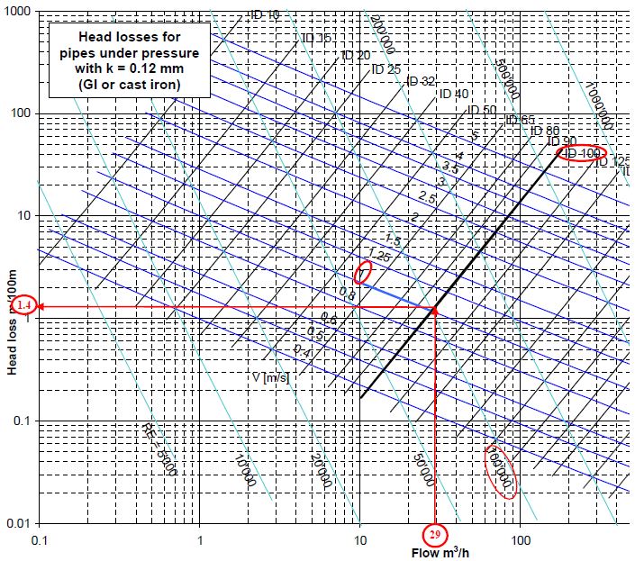Fig 4- 7 Head losses for pipe under pressure

Charts for other roughness are given in the annexe.

Tables for friction losses coefficients 

Several documents still give Tables for friction losses coefficients, they were done for calculator and should not be used any more as they are not precise at all and give wrong impression of precision.
Computer can easily make all necessary calculations; it will be more precise and much simpler to iterate.

4.9. System curves

As it has been shown (eq.4-11), head losses depend on one hand on the system (punctual and linear losses) and on the other hand on the flow. Thus, hLP could be calculated for given water scheme for different flows, and represented in a chart as the example in the side.
The curve is close to a parabolic function but not exactly as the linear losses depends also
on the velocity. In the attached chart, the flow coincides with the velocity. The head losses coefficient used to draw the parabolic curve is the value obtain with a velocity of 1 m/s (in the middle of the curve). As it can be seen, the curves diverge quickly after 1.3.
This concept will be used later to define the working point of a system with pump.

Basic exercises

1. What are the ID, the SDR and the Series of a pipe with an outside diameter of 110 mm and a
thickness of 6.6 mm?
2. What is the nominal pressure of this pipe if it is made with PVC and used at a temperature of
30°c? If it is made with PE80, PE100 at 20°C?
3. What is the nominal pressure of these PE pipes if it is used for gas (the service ratio is 2 for
gas)?
4. What are the friction losses in a DN150 PVC pipe of 2.2 km, with a velocity of 1 m/s? Same
question for a steel pipe (k=1mm) (can be estimated with charts in annexes)?

Intermediary exercises

5. What is the hydraulic diameter of a square pipe (b=h)? Of a flatten (elliptic) pipe with b=2h?
6. What is the minimum velocity and flow that should flow to avoid air pocket (Re = 10'000) in a
pipe of DN25, DN200, DN500 ?
7. What is the punctual friction losses coefficient for a pipe connected between to tanks, with four
round elbows (d=D), a gate valve, a non-return valve and a filter?
8. What is the average punctual friction losses coefficient for the accessories of a DN200 pump?
9. What are the friction losses in a DN150 PVC pipe of 2.2 km, with a velocity of 1 m/s? Same
question for a steel pipe (k=1mm) (to be calculated with equations, not estimated with charts)?
10. What should be the diameter of an orifice to create losses of 20 meters in a DN100 pipe with a
velocity of 1 m/s?

Advanced exercises

11. What is the flow in a DN150 steel pipe of 800 m connecting two tanks with a gate valve, five
elbows and a filter, if the difference of height between the tanks is 2m; 5m; 10m?
12. How much shall a pipe be crushed to reduce the flow by half?
13. What is the flow when the pipe is crushed to half of its diameter?

References for this chapter:

KSB : Selecting Centrifugal Pumps